Influence diagnostics for linear regression in Excel

This tutorial explains how to compute and interpret influence diagnostics for linear regression in Excel using XLSTAT software.

Dataset for a linear regression with influence diagnostics

The data have been obtained in Lewis T. and Taylor L.R. (1967). Introduction to Experimental Ecology, New York: Academic Press, Inc.. They concern 237 children, described by their gender, age in months, height in inches (1 inch = 2.54 cm), and weight in pounds (1 pound = 0.45 kg).

Goal of this tutorial

Before proceeding to a statistical modelisation, you might be looking for identifying observations which represent extremes values (outliers) of the different variables in order to exclude them from the analysis. However, this procedure doesn’t give you any indication about how such an observation can influence the estimation of the model’s parameters. In order to evaluate this, it is suggested to compute the influence diagnostics for those observations.

Setting up a linear regression with influence diagnostics

After opening XLSTAT, select the XLSTAT / Modeling data / Regression function.

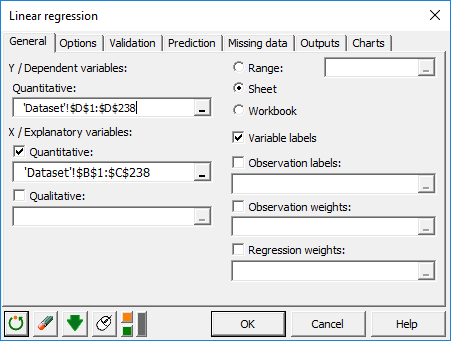
Once you've clicked on the button, the Linear Regression dialog box appears.

Select the data on the Excel sheet. The Dependent variable (or variable to model) is here the "Weight".

The quantitative explanatory variables are the "Height" and the "Age".

As we selected the column title for the variables, we leave the option Variable labels activated.

Note: for more details on how to set up a linear regression in Excel using XLSTAT, check out our tutorial

Interpreting Influence diagnostics of a linear regression

Several indicators are computed. Among the influence diagnostics, we can find the Leverage, the Mahalanobis distance, the Cook’s D, the CovRatio, the standardized DFFits, and the standardized DFBetas. The majority of these indicators measure differences between models with or without the ith observation (the difference in prediction, parameters estimation, variance-covariance matrix …)

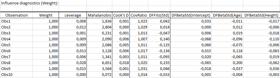
Here, we will focus on the interpretation of the standardized DFFits and DFBetas.

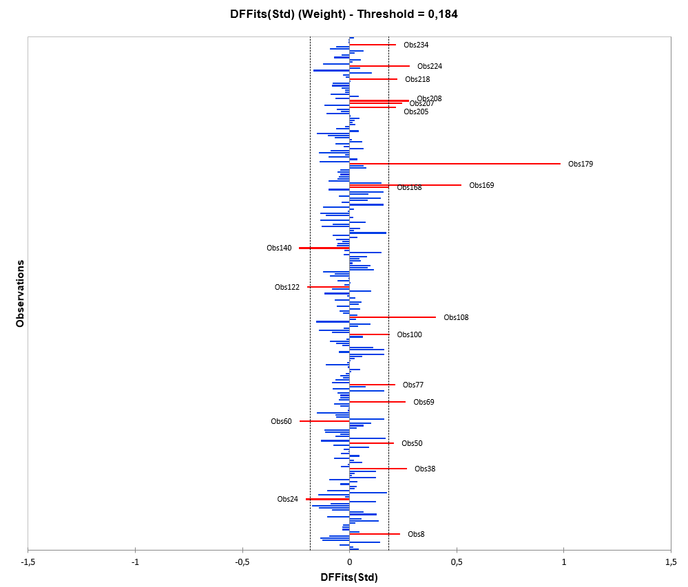
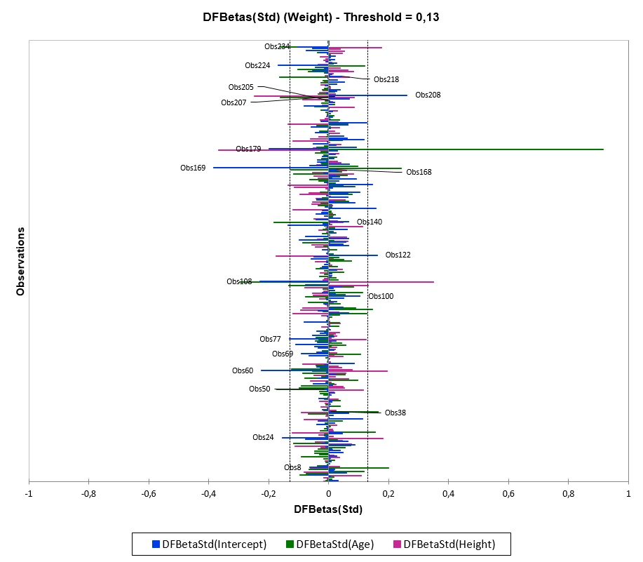
We observe a strong influence of the 179th observation on the estimation of the parameters and on the predictions. The following observations has also an effect (weaker) : 8, 24, 38, 50, 60, 69, 77, 100, 108, 122, 010, 168, 169, 205, 207, 208, 218, 224 and 234. The individual 179 measures 67.5 inch for 171.5 pounds (77kg). If we look more in details at the characteristics of this individual, he is 20 years old, contrary to the other interviewed children who are between 13 and 14. His weight/height ratio is around 2.5, whereas it is 1.65 on average for the whole sample. Among all parameters, he has a stronger influence on the estimation of the Age. Indeed, his age is more outlying than its height. Based on the above observations, we suggest to exclude this individual from the model.