Apprentissage d'une régression par machines à vecteurs de support dans Excel

This tutorial shows how to perform and interpret a Support Vector Regression (SVR) in Excel using the XLSTAT software.

Dataset for SVR

The dataset named abalone contains characteristics of abalones, marine gastropod molluscs. To predict the age of an abalone, one needs to color the rings and count them through a microscope, which is a time consuming-task. That is why, we want to predict the age of abalones with measures which are easier to obtain.

Goal of this tutorial

The goal of this tutorial is to learn how to set up and train a SVR on the Abalone dataset and see how well the regression performs on a validation set.

Setting up a SVR in XLSTAT

Once XLSTAT is open, click on Machine Support Vector as show below:

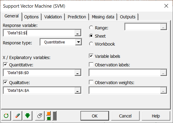
Once you have clicked on the button, the SVM dialog box appears. Select the data on the Excel sheet.

In the Response Variable field, select the quantitative variable you want to predict. In our case, this is the column giving the number of rings.

In order to fit a regression, select Quantitative as response type.

We also select both quantitative and qualitative explanatory variables by checking both checkboxes as shown below.

In the Quantitative field, we select columns corresponding to the following fields: - Length,

• Diameter,
• Height.

In the Qualitative field, we select the column with qualitative information: Sex.

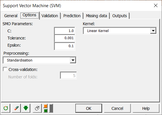
As the name of each variable is present at the top of the table, we must check the Variable labels checkbox. In the Options tab, the regressor parameters are set up. For the SMO parameters, we leave the default options. The C field corresponds to the regularization parameter. It translates the amount up to which deviations larger than ε are tolerated. In our case, we set the value of C at 1, but C has to be positif.

The tolerance parameter indicates how accurate the optimization algorithm will be when comparing support vectors. If you want to speed up calculations, increase the tolerance parameter. We leave the tolerance at its default value.

The Epsilon field is the parameter which specifies the epsilon-tube and affects the number of support vectors selected. Again, we leave epsilon at its default value but has to be positif.

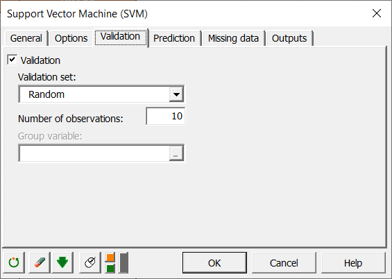
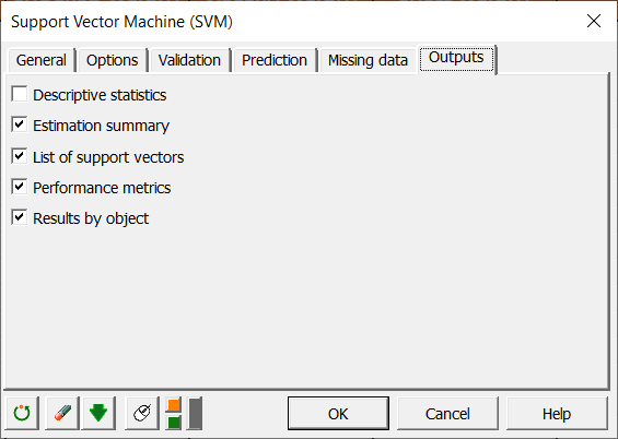
We select Standardisation in the preprocessing field and we use linear kernels as shown below. As we want to see how well our regression model performs, we will make a validation sample out of the training sample. For this purpose, in the Validation tab, we check the Validation checkbox and select 10 observations randomly drawn from the training sample as indicated below. Finally, in the Outputs tab, we select the outputs we want to obtain as shown below:

Interpreting the results of the SVM regressor

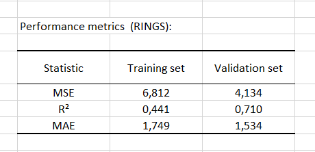
The first table displays performance measures and evaluates the regression. Here, we use the mean squared error, mean absolute error and the coefficient of determination. We want a low mean squared error, a low mean absolute error and a coefficient of determination near 1.

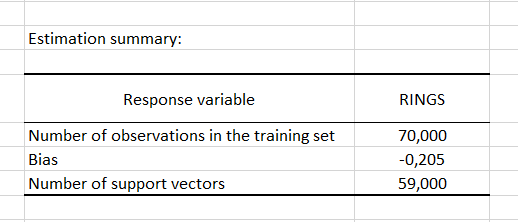
The coefficient of determination for the validation set has a correct score of 71%. The second table displays a summary of the optimized SVR. You can see on the figure below that there were 70 observations used to train the regressor out of which 59 support vectors have been identified. Finally, the bias, which is the origin of the hyperplane, will be used during the prediction of the validation sample. 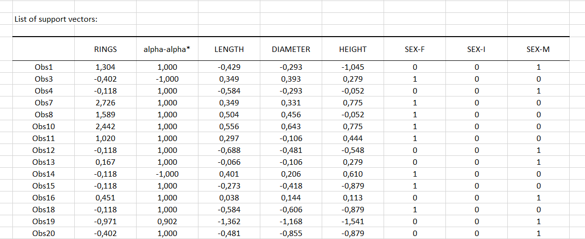The next table shown below gives the complete list of the 59 supports vectors with the associated alpha-alpha* coefficient values, values of the response variable, scaled explanatory variables and the disjunctive matrix of qualitative variables. 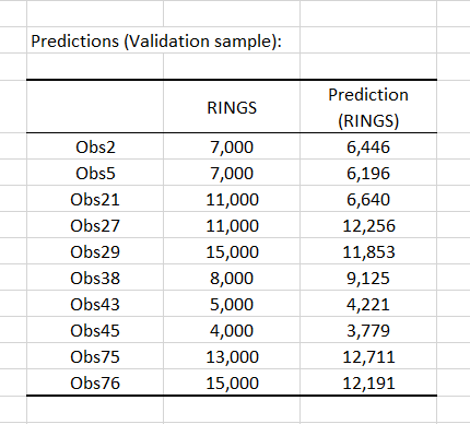Finally, you can see predicted values obtained by the regression for each observation on the figure below: